Creating AI for Artificial Worlds

Motivation

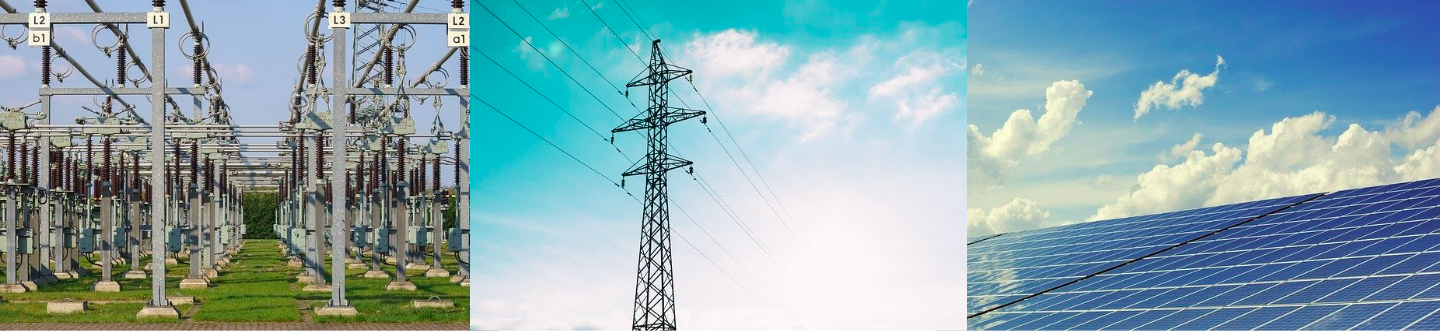
Energy Access Planning

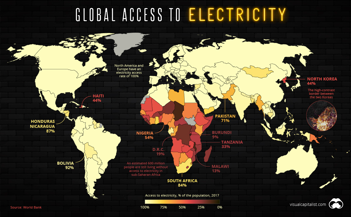
Access to clean and affordable energy (one of the seventeen UN Sustainable Development Goals) is becoming increasingly critical, especially for promoting economic development, social equity, and improving quality of life. Further, it has been shown that electricity access is correlated with improvements in income, education, maternal mortality, and gender equality. Yet, worldwide, 16% of the global population, or approximately 1.2 billion people, still don’t have access to electricity in their homes. This map from the World Bank in 2017 highlights the uneven distribution of energy access, with the majority of those without electricity access concentrated in sub-Saharan Africa and Asia.

Image from: https://www.visualcapitalist.com/mapped-billion-people-without-access-to-electricity/

One of the first steps in improving energy access is acquiring comprehensive data on the existing energy infrastructure in a given region. This includes information on the type, quality, and location so that energy developers and policymakers can then strategically and optimally deploy energy resources. This information is key for helping them make decisions about where to prioritize development, and whether they should use grid extension, micro/minigrid development, or offgrid options to bring electricity access to new communities.

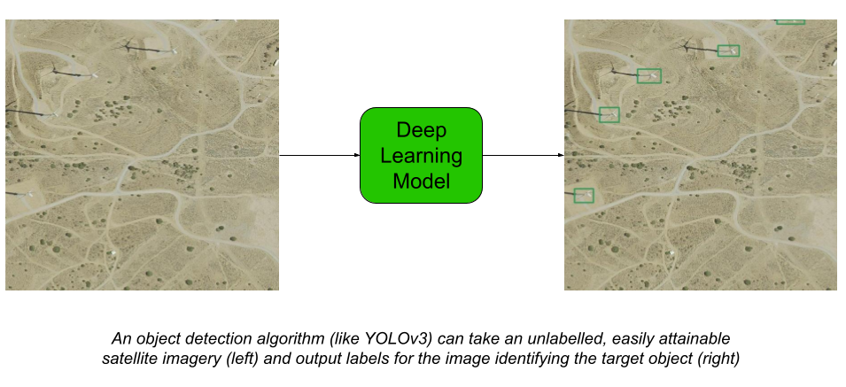
However, this critical information for expanding energy accessibility is often unattainable or low quality. A solution to this issue is to automate the process of mapping energy infrastructure in satellite imagery. Using deep learning, we can input satellite imagery into an object detection model and make predictions about the characteristics and contents of the energy structure in the region featured in the image, providing energy experts with the necessary data to expand electricity access.

Object Detection

Image from: ResearchGate

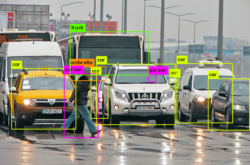
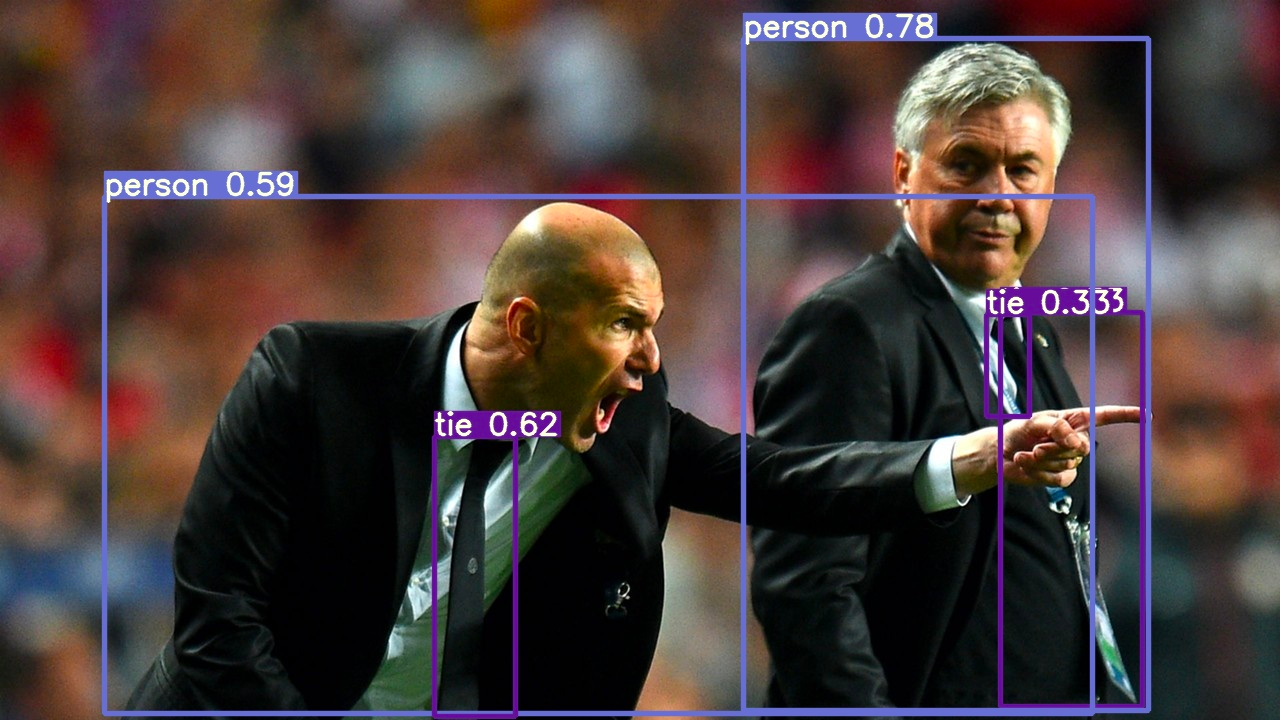
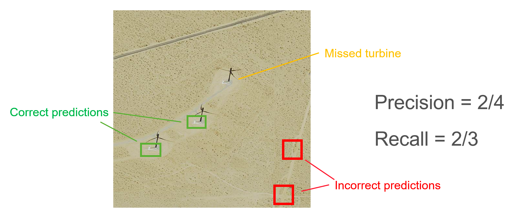
Object detection consists of classification (identifying the correct object) and object localisation (identifying the location of a given object). Our project has a particular emphasis on object detection, as we seek to improve the detection of energy infrastructure in different terrains as a part of expanding energy access data. Object detection models analyze the scenery of photos and generate bounding boxes around each object in the image. In doing so, it classifies each object and assigns a confidence score based on the accuracy of its prediction. The model predicted that each of the green, yellow, orange, and pink boxes in the image on the left would indicate different objects, being a truck, a car, an umbrella, and a person. Based on examples provided to it, the model learns how to predict these boxes and classes. We refer to these labeled images as ground truth as they contain boxes that denote every object's class and the location within the image.

Applying Deep Learning to Overhead Imagery

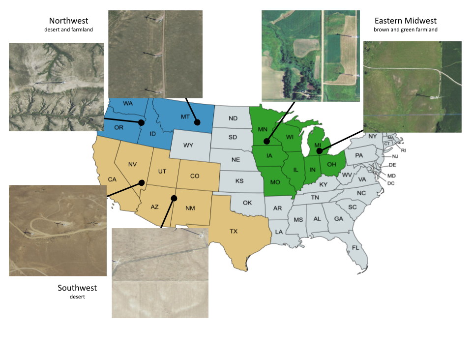
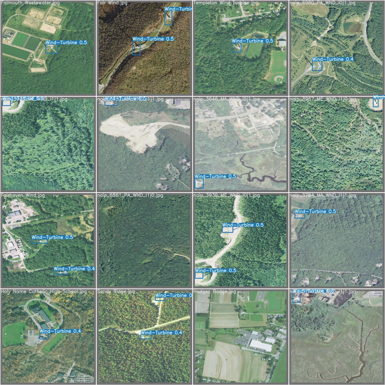
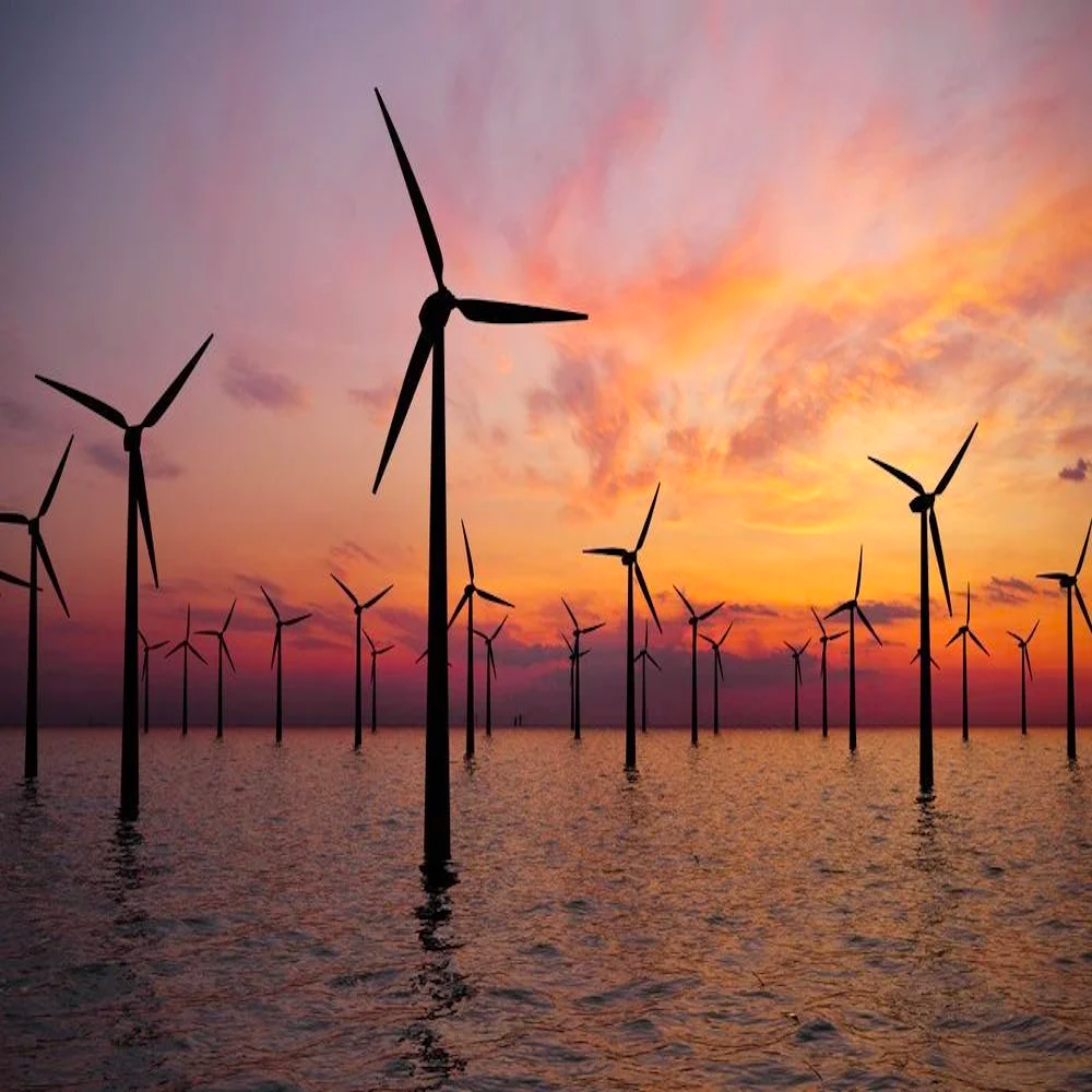
After training our object detection model, we can apply it to a collection of overhead imagery to locate and classify different energy infrastructure across entire regions. In our experiments, we test our ability to detect wind turbines to maintain consistency with previous experiments. While we could demonstrate energy infrastructure detection for any number of types of electricity infrastructure, wind turbines were chosen due to their relatively homogeneous nature as opposed to different power plants and other energy infrastructure. Additionally, our dataset was limited to the US, as there is a wealth of high resolution overhead imagery available throughout the US. Ultimately, the methods used to improve object detection of energy infrastructure will be expanded to more energy infrastructure and tested on more regions, however, limiting the the infrastructures to wind turbines and using readily available US imagery helps to quickly provide performance benchmarks for our real and synthetic datasets.

Challenges with Object Detection

Problem 1: Lack of labeled data for rare objects

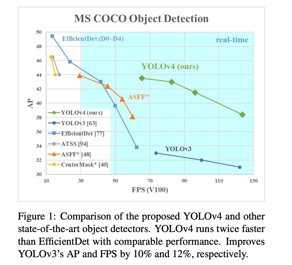
While the potential of object detection seems promising, it presents two main challenges. The first is that properly training the object detection model requires thousands of already labeled images (images in which the location of the target object is known and identified via an annotation). According to Alexey Bochkovskiy, developer of the highly used and precise YOLOv4 object detection model, it is ideal to have at least 2000 different images for each class to account for the different sizes, shapes, sides, angles, lighting, backgrounds, and other factors that could vary from image to image. Thus, in order to make the object detection model best generalize, the model will require 1000s of training images per energy infrastructure. Because many types of energy infrastructure are rare objects, obtaining and annotating such a large quantity of satellite images featuring these infrastructures manually is expensive in terms of both time and cost.

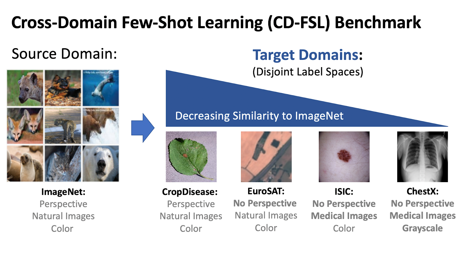
Problem 2: Domain adaptation

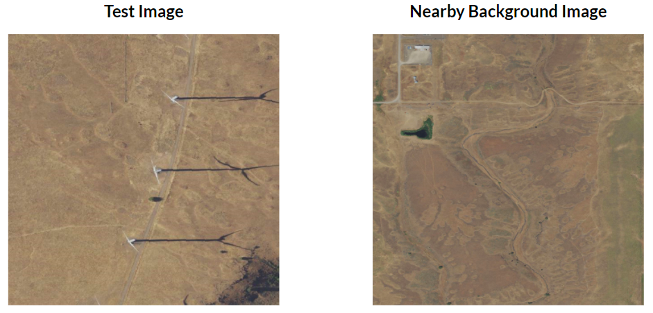
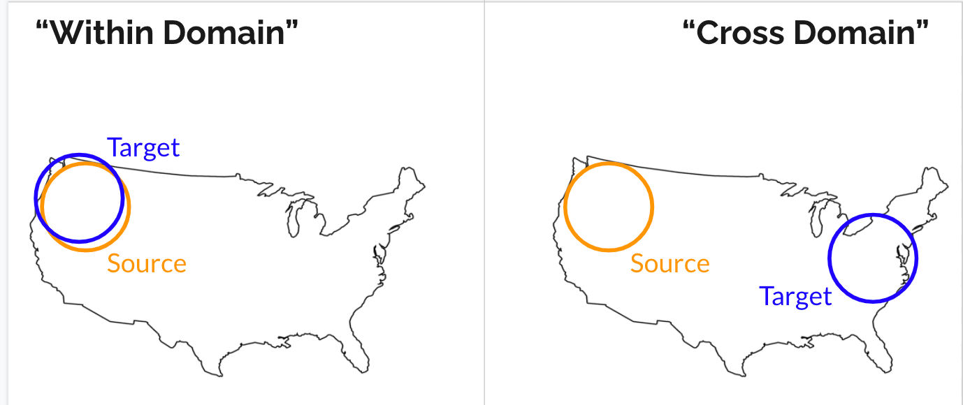
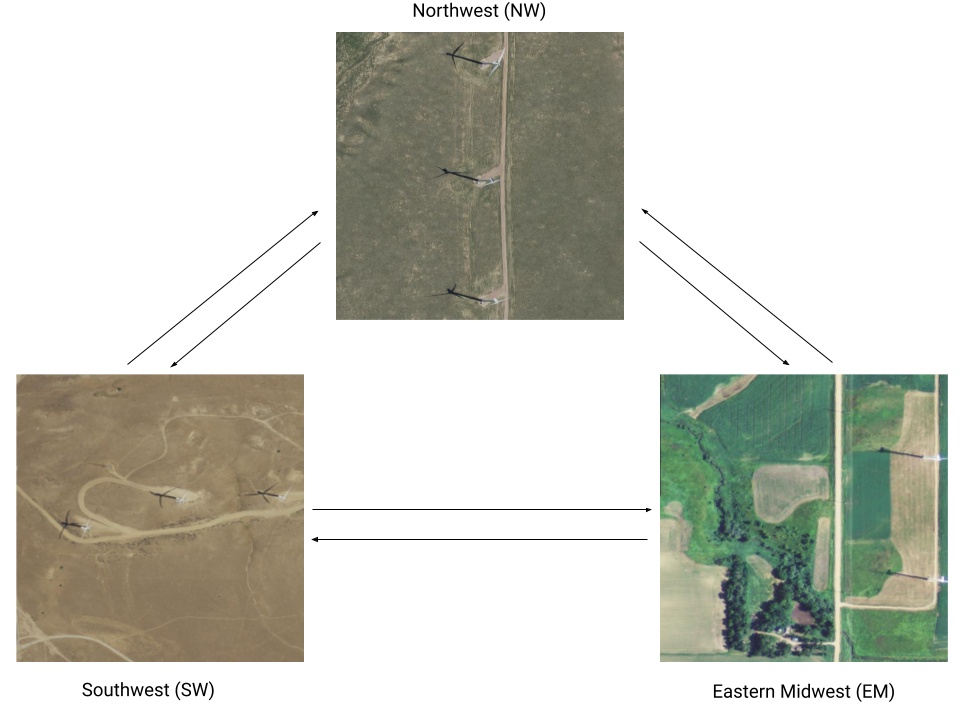
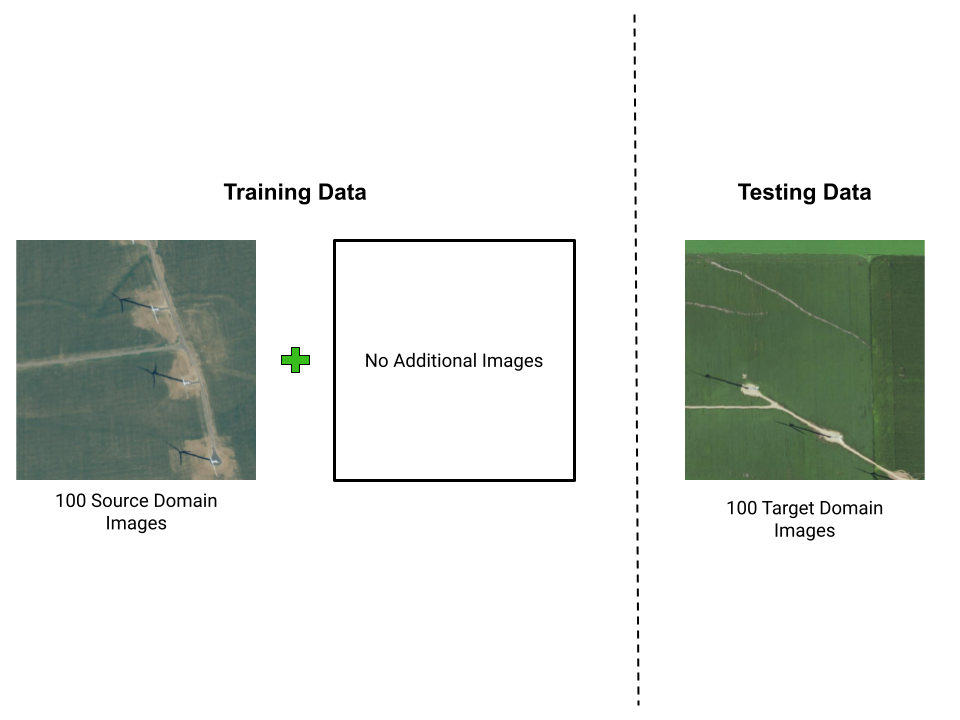
The second challenge we face is that in training an object detection model to detect energy infrastructure in certain regions, our training set and testing set must come from different locations and thus may have differences in geographical background and other environmental factors. Without being properly trained for the test setting, object detection models are not great at generalizing across dissimilar images yet. What this means is that if we train our model on a collection of images from one region, featuring images with similar background geographies, the model will then be able to perform fairly well on other images with those same physical background characteristics. However, if we then try to input images from a different region with different geographic characteristics, the model's performance becomes significantly worse, since it hasn’t been trained with images containing those specific background features.

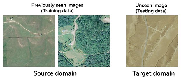
Figure: Example of the domain adaptation challenge, for a model trained on images with geographical features of the images in the source domain (forest & grasslands) that underperforms when tested on images with different background in the target domain (desert)
Image from: 2020-2021 Bass Connections team.

Proposed solution: Synthetic Imagery

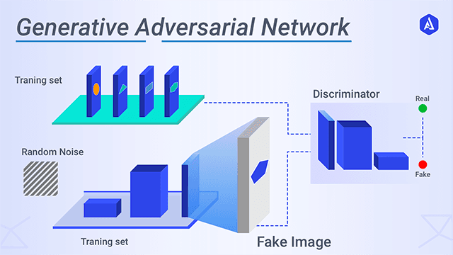
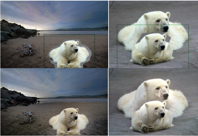
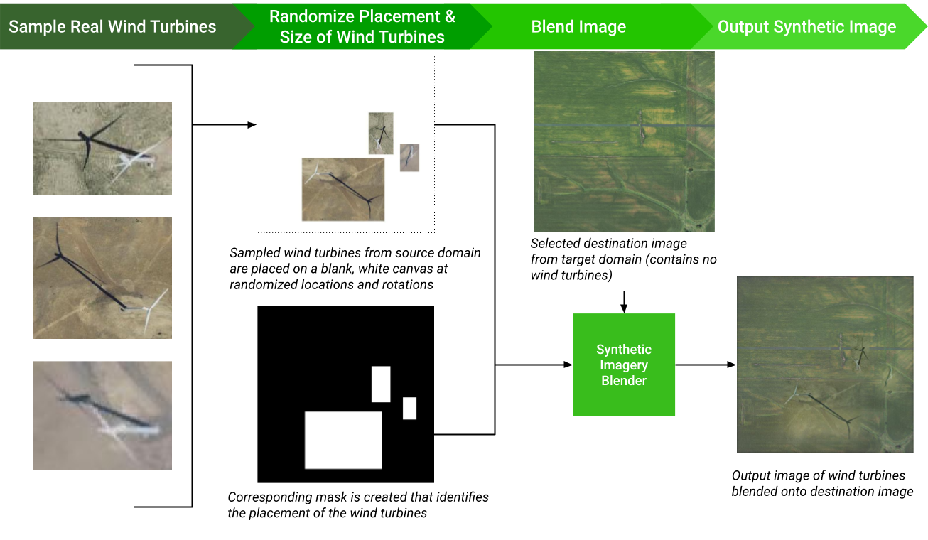
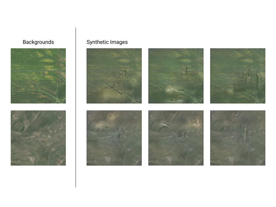
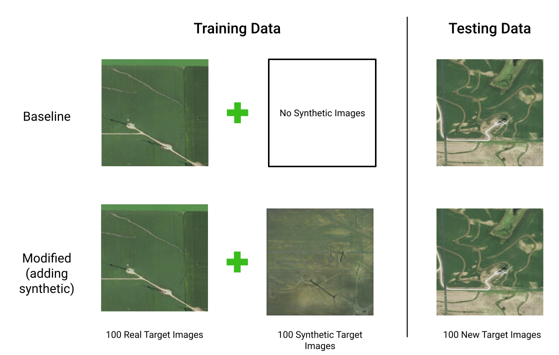
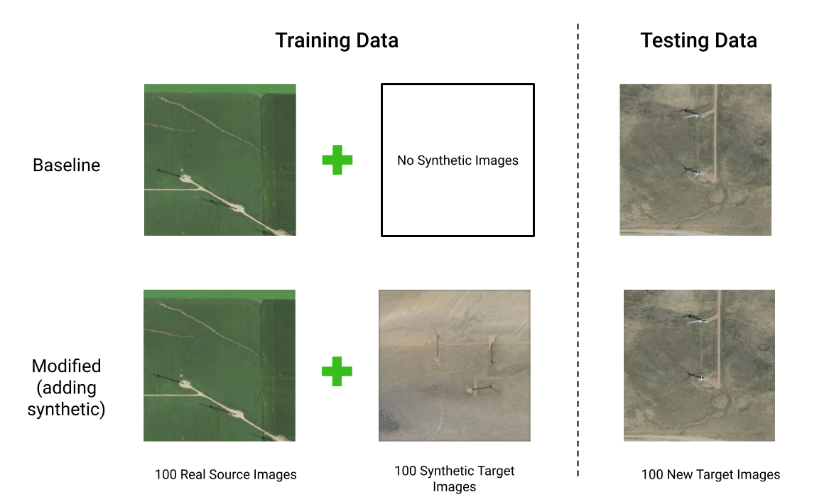
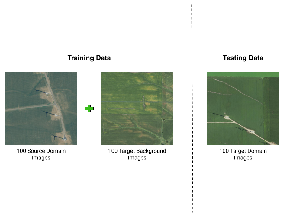
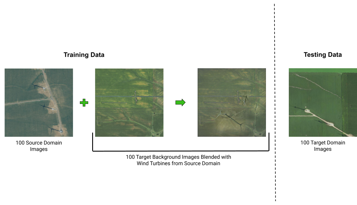
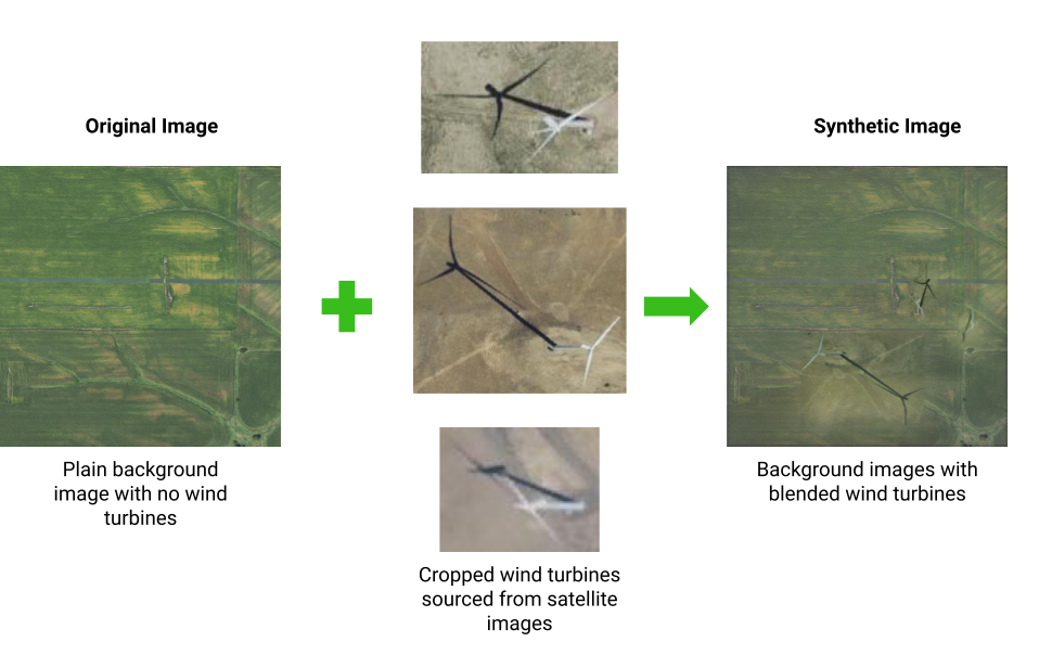
Our proposed solution to address these two problems is to introduce synthetic images into our training dataset. These synthetic images include a labeled target object implanted into the background of the target domain, so that even if we don’t have real labeled images from the target domain, we can create close imitations.. The synthetic images supplement the original real satellite imagery dataset to create a larger dataset to train our object detection model, diversifying the geographical background and orientation of energy infrastructure that the model sees. We generate these synthetic images by cropping the energy infrastructure out of satellite images and using a Generative Adversarial Network to blend them into a real image without any energy infrastructure from one of the target geographic domains.

Figure: Synthetic imagery generation process overview

Previous work

For five years, the Duke Energy Data Analytics Lab has worked on developing deep learning models that identify energy infrastructure, with an end goal of generating maps of power systems and their characteristics that can aid policymakers in implementing effective electrification strategies. Below is a timeline of our team's progress.

2015-2016

Our Humble Beginnings

In 2015-16, researchers created a model that can detect solar photovoltaic arrays with high accuracy [2015-16 Bass Connections Team].
2018-2019

Transition to New Infrastructures

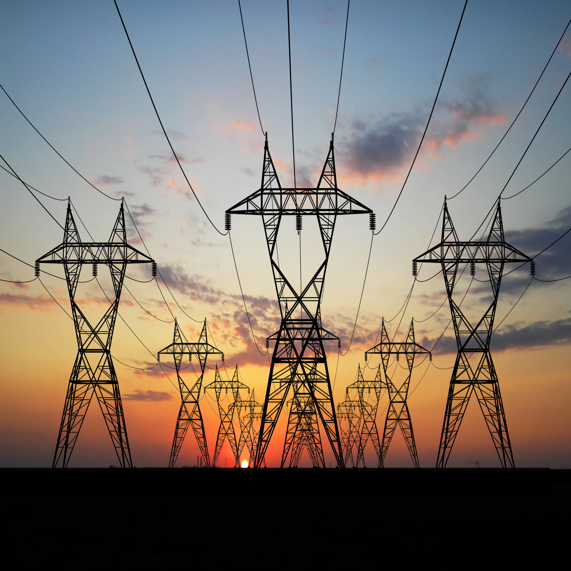
In 2018-19, this model was improved to identify different types of transmission and distribution energy infrastructures, including power lines and transmission towers [2018-19 Bass Connections Team].
2019-2020

Expanding Our Geography

Last year's project focused on increasing the adaptability of detection models across different geographies by creating realistic synthetic imagery [2019-20 Bass Connections Team].
July 2020

Improving Our Perfomrnace

In 2020-2021, the Bass Connections project team extended this work, trying to improve the model’s ability to accurately detect rare objects in diverse locations. After collecting satellite imagery from the National Agriculture Imagery Program database and clustering them by region, they experimented with generating synthetic imagery by taking satellite images featuring no energy infrastructure and placing 3D models of the object of interest on top of the image, and capturing a photo that mimicked the appearance of a satellite image [2020-21 Bass Connections Team]. Their paper, Wind Turbine Detection With Synthetic Overhead Imagery, was published in 2021 by IGARSS.
Now

Our Work

In our project, we build upon this progress and try to improve the 2020 Bass Connections team and 2021 Data Plus team's ability to enhance energy infrastructure detection in new, diverse locations.

Key Contributions

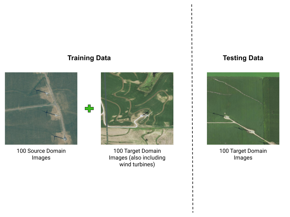
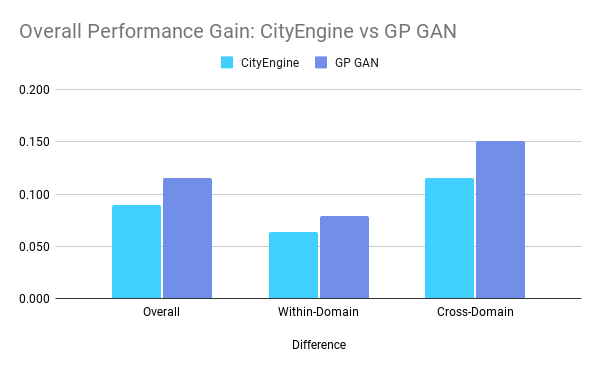
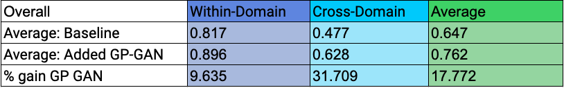
We propose a new method for unsupervised domain adaptation that is comparable to state-of-the-art domain adaptation techniques and methods. We created a large, diverse, publicly-available dataset for wind turbine and transmission tower object detection. Our dataset encompasses 5 large geographic regions of the United States, and is the first of its kind for both wind turbines and transmission towers. We found that adding unlabeled background imagery was beneficial to the object detection performance of neural networks in the context of domain adaptation with remote sensing data.

Methodology

Below is a description of the experiments we conducted to evaluate if adding synthetic images to an object detection algorithm enhances its performance across geographic domains. After gathering real images and generating synthetic images, we can construct four datasets. The first dataset includes only real imagery, the second dataset includes both real and our synthetic images. We can train an object detection model on the first dataset, test it, and then repeat the process with the second dataset, comparing the results. If the model performs better when trained on a dataset with synthetic imagery, we can conclude that the synthetic imagery aids the model's performance.

In addition to these comparisons, we perform additional experiments comparing the quality of our synthetic data as supplemental data to the baseline by evaluating the performance of a third dataset with supplemental unlabeled target imagery and a fourth dataset with labeled target imagery. This helps us identify the relative quality of our synthetic data compared to true target data. Finally, we can compare our technique to state-of-the-art domain adaptation techniques, to determine the usefulness of our technique compared to other solutions to the domain adaptation problem.

Collecting Real Imagery

To ensure our experiments are employed on a range of imagery from different geographies, we defined three domains, or geographical regions, in the US. These are as follows: Eastern Midwest (EM), Northwest (NW), and Southwest (SW). Each of these domains are visually distinct, varying in characteristics such as color distribution and terrain among other geographical features. Overhead satellite imagery of various target objects (wind turbines, transmission towers, and ____) in each region have been collected from the National Agriculture Imagery Program (NAIP). Images from NAIP cover a large part of the US and are very high resolution, making it suitable for our experiments. Below we can see the regions splits by which states they include, as well two images we collected for each region.

Figure: Map of the U.S. showing the U.S. states and 2 images we collected in each region

Creating Synthetic Imagery

GANs Overview

Generative Adversarial Networks (GANs) are a method of generative modeling. The concept behind GANs is a zero sum game between two Neural Networks- a generator network and a discriminator network. While the generator attempts to create images that are as realistic as possible, the discriminator tries to determine if those images are real or fake. The generator then learns from what the discriminator identifies as fake, helping it create more realistic images. This novel approach to generative modeling has seen a rapid increase in usage in various scientific domains, due to its ability to generate photorealistic images for tasks including data augmentation, creating art, image to image translation, image harmonization, and image super-resolution.

Image from: Akira.AI

Figure: Top displays polar bear being cut and paste from the left image to the right image. Bottom displays polar bear in the left image being blended with the GP GAN into the right image.

GANs for Image Blending

In trying to generate synthetic imagery with real wind turbines in new terrains, our problem presented the need for image harmonization and image blending. This consists of matching the visual appearance/style of the wind turbine and geographical background images when blending them into a single image. Given the GANs state-of-the-art performance in “GP-GAN: Towards Realistic High-Resolution Image Blending” by Huikai Wu, et al., we chose to investigate the potential for GANs to realistically develop our synthetic imagery dataset.

Synthetic Imagery with GP GAN Pipeline

Synthetic images produced by the GP-GAN are a quick and cost-effective solution to labeled datasets that are incommensurate with the great training set size required for adequate performance. To produce our synthetic images, we automatically crop all energy infrastructure in the source training data and perform copy-paste augmentation of these images on a white background, in randomized locations, sizes, and rotations. In performing the crop, we ensured the preservation of key features including the shadow around the target object, which can be a helpful tool within the receptive field of an object detection model for identifying the infrastructure of interest. The mask with the energy infrastructure is then blended onto a background image (does not contain any energy infrastructure) from the data-scarce target domain using the GP-GAN model. Each image is blended in approximately 7 seconds, making our data pipeline an incredibly quick and resource efficient solution for data scarcity. For reference, we created a dataset of approximately 1600 images in approximately 3 hours holding almost 200 images for 9 different combinations of source and target domains. Each synthetic image featured a unique combination of background image, source turbines, and randomized location, rotation, and size, creating a diverse set of supplemental imagery. Below are some example synthetic images created from a variety of background images.

Figure: Our synthetic images contain a variety of background images, source turbines, and turbine orientations.

Synthetic Imagery Design Considerations

In designing the synthetic imagery, we must be careful in controlling environmental variables to generate a diverse dataset of images that are close to real images. These design considerations are critical components of our methodology as the closer the synthetic imagery is to the real test imagery, the more the synthetic imagery will improve our performance when adding it to our training set.

Figure: Bounding box size distribution of turbines in real imagery.

Custom Image Augmentation

The first step of our image generation pipeline is our custom image augmenter, which performs copy-paste augmentation of wind turbines onto a white canvas, which will be blended with a background via the GP GAN to create our synthetic imagery. In performing this augmentation, we must consider the location, size, rotation, and density of our synthetic turbines. A key benefit of our model is the ability to customize these distributions to provide maximal benefit. We first investigated the distributions of the real training data to explore how to make the most realistic synthetic data. In creating our augmented images, , we then sampled real turbines from the source domain training data, applied a random location and rotation to the turbine, and placed them onto the canvas. We placed 3 turbines per augmented image, as 3 represents the 90th percentile of the number of turbines in our real training data, and allows us to create dense synthetic data to provide more target objects for the model to learn. In randomizing location and rotation and creating denser synthetic images, we allow the object detection model to become familiar with many wind turbines from various contexts, angles, and views.

Which Background Images to Use

Additionally, we had to choose which background images to have placed under our synthetic wind turbine models. We chose to use background imagery regionally close to the real images in our testing set to maximize the similarity of our synthetic imagery with the target data. This methodology is consistent with real scenarios, as we will likely have access to unlabelled imagery or have the ability to collect unlabelled imagery from around the region we wish to test on for use as background images. Given the lack of manual labeling and filtering required as well as our ability to generate many sources to blend with each background image, this background data collection would ideally not be too time consuming. Using the background images close to our testing locations allows us to estimate the potential performance increase that the synthetic data can provide without introducing confounding variables such as a mismatch between the synthetic background image domain and the target domain (which makes it difficult to attribute poor performance to the different geographic context or synthetic data generation).

Figure: Test image and nearby collected background image.
Image from: 2020-2021 Bass Connections team.

Experimental Setup

Overview

To evaluate the potential of synthetic imagery in improving the performance of object detection, we set up within and cross domain experiments, where a domain is defined as a specific geographic region. The source domain refers to the region that the real training data comes from, while the target domain refers to the region that the object detection model is applied to. These two types of experiments each correspond to a potential real-world situation one might encounter, and help us to evaluate the potential performance of the object detection model in each of these situations.

In the context of energy access planning, the ultimate goal of this project is to utilize object detection in various regions of the world where energy access is extremely limited and information on existing energy infrastructure is not readily available. Thus, the object detection model must be able to generalize well across different images despite labeled real satellite imagery most likely being limited.

Figure: Overall Experiment Setup. In within-domain experiments, the target domain (Northwest) remains the same geographic region as the source domain (Northwest). In cross-domain experiments, the target domain (Northeast) has no labeled real data, so the model is trained on a different source domain (Northwest) and then applied to the target domain. Orange color denotes a source domain, whereas blue color denotes a target domain.
Image from: 2020-2021 Bass Connections team.

Figure: Pairwise experiment setup. The arrow tails point toward the source domain (where real training data comes from), whereas the arrow heads point toward the target domain (where the model will be tested on). Bi-directional arrows indicate each domain serves as the source for testing the other two domains, and in a separate experiment, the same domain serves as the target to be tested using model trained on the other domains.

Our within-domain experiments, where the source and target domains are within the same geographic region, will help us to evaluate the potential for synthetic imagery to supplement limited real training data.

However, as mentioned previously, one of the key challenges that object detection presents is its poor performance when applied to data that looks significantly different from the data on which it is trained. Thus, the cross-domain experiments reflect the potential situation where there exists no data at all from the target domain, and thus the object detection model must be trained on data from an entirely different region. For this experiment, the synthetic data that is used will come from the target region, but the real images will come from a source region, different from the target.

Optimizing the Ratio of Real to Synthetic Data

In constructing our experimental datasets, we need to figure out what ratio of real to synthetic data yields the largest gain in performance (if any). Introducing too much synthetic data could lead to overfitting to synthetic data and any irregularities within the synthetic data or differences with regular images would be exacerbated such that the object detection model may perform worse. However, adding too little synthetic data will have a negligible effect on performance. Thus, in creating our synthetic data, we created a large pool of supplemental data for each domain combination, including 100 supplemental images with unique backgrounds and randomly sourced turbines. We then conducted an experiment by varying the mixed batch ratio used with YOLOv3. Given a batch size of 8, the mixed batch ratio determines how many of these 8 images will be from the synthetic images, and how many will be from the source real images. In experimenting with different ratios with our synthetic data generation process, we are now able to better identify how the performance boost of our synthetic imagery changes when adding more and more synthetic imagery. In the experiment, we found that —Results—. However, in order to not bias our results towards what works best for our technique, we used a mixed batch ratio of 1 throughout all of our comparative experiments, as this is the smallest ratio that includes synthetic images and will allow for a fair comparison of the initial benefit provided by adding synthetic images, without biasing the results as different techniques could yield better results as the ratio changes.

Image from: 2020-2021 Bass Connections team.

YOLOv3

Figure: Sample output image from Ultralytics YOLOv3 GitHub repository.

YOLOv3 is a popular object detection model used in various computer vision tasks. YOLO stands for You Only Look Once, as the model is only applied to an image once, dividing the image into regions and predicting bounding boxes for each region in the image. It is widely used because of its much faster object detection speed with similar mAP as other well-performing models. This speed is important for our task as ultimately, we hope to automate the mapping of satellite imagery to energy infrastructure, which will require the model to quickly identify infrastructure in large datasets including imagery of entire regions. Our previous Bass Connections team also used YOLOv3, such that we used YOLOv3 to make direct comparisons between the performance of our models and their's without confounding variables.

Figure: Within-domain experiment example using Northwest as target domain.

Within Domain Experiment (Target = Source)

For each of the domains we selected, we ran the baseline and modified experiments, where all of the data came from the same region. This experiment helps to evaluate the overall ability of synthetic imagery (especially using our GP-GAN technique) to improve the object detection performance.

Figure: Cross-domain experiment example using Northeast as target domain and Eastern Midwest as non-target domain.

Cross Domain Experiment (Target not equal to Source)

For these experiments, the domains for the real source and target images are different, while the synthetic images used in the modified training dataset are from the target region. Thus, with synthetic images more similar to the target region, we hypothesize that the addition of the synthetic images will improve the accuracy of the object detection when the target and source regions are dissimilar in appearance. These experiments will help us to evaluate the potential for synthetic imagery to improve the object detection model’s ability to generalize across different regions despite the limitations of the existing training data.

Design Setup

Having sampled our data and found the optimal real to synthetic ratio, our final datasets for each region is:

Baseline: Train on 100 Real Non-Target Images, Test on 100 Target Domain Images
Modified: Train on 100 Real Non-Target Images + 100 Syn Target Images, Test on 100 Target Domain Images
Lower bound: Train on 100 Real Non-Target Images + 100 Real Unlabeled (Background) Target Images, Test on 100 Target Domain Images
Upper bound: Train on 100 Real Non-Target Images + 100 Real Labeled Target Images, Test on 100 Target Domain Images

Baseline Experiment

Baseline Experiments: There was no augmentation of training data in the baseline experiments; the model was trained on 100 real satellite images from the source domain, and then tested on 100 real images from the target domain. In the context of these experiments, “real images” refer to satellite images that naturally contain the target object.

Figure: Baseline experiment example using Northwest as source domain and Eastern Midwest as target domain.

Lowerbound Experiment

For the second set of experiments, the training dataset is made up of the original 100 real source domain images in addition to 100 background satellite images from the target domain that contained no target objects. The model was tested on the same 100 real target domain images. The motivation behind this set of experiments was to evaluate the relative improvement that the background context of the target domain could bring to the performance of the model. These background images, although lacking objects of interest, are often easier to obtain and don’t require any manual labeling.

Figure: Lowerbound experiment example using Northwest as source domain and Eastern Midwest as target domain.

Upperbound Experiment

The third set of experiments served as an “upper bound” for the other three experiments to help evaluate the relative performance gain brought by synthetic image augmentation. In these experiments, the original 100 real source domain images were augmented with 100 additional real images from the target domain. These additional real images contained wind turbines and were labeled. This experiment simulates the ideal scenario - increasing the total amount of relevant training data for the algorithm, but in a real world context, obtaining those additional 75 labeled images from the target domain may be incredibly hard and expensive.

Figure: Upperbound experiment example using Northwest as source domain and Eastern Midwest as target domain.

Synthetic Experiment

Finally, the last set of experiments were our main focus as they included the addition of 100 of our GP-GAN synthetically generated images from the target domain to the training dataset. We expect to see significant improvement in performance with the addition of synthetic images in comparison to both the baseline and the addition of background images.

Figure: Synthetic experiment example using Northwest as source domain and Eastern Midwest as target domain.

Figure: Cross-domain experiment example using Northwest as target domain and Eastern Midwest as non-target domain.

Full Experimental Setup

All in all, this creates a four-fold experiment structure, in which we compare our synthetic data to the baseline (without synthetic data), background imagery without our turbines planted in, and real imagery from the target domain. Evaluating the relative performance of our technique among these experiments allows us to identify the benefit of our technique in terms of bridging the benefit between dataset size that comes from adding background imagery to the ideal case of real labeled images that come from target domain.

Results

Figure 1: In this image, the YOLOv3 model predicted that 4 objects were wind turbines. 2 of those predictions were correct, meaning the precision would be 2/4. There are 3 wind turbines in the image and the model found 2 of these, meaning the recall would be 2/3.
Image from: 2020-2021 Bass Connections team.

Performance Metrics

Before evaluating our results, it's critical that we first understand the metrics that we have chosen to measure performance. The primary metrics we will use is Average Precision, which combines the classification metrics of precision and recall. We will explain the implication of these metrics starting with the images on the left.

Precision: Out of the areas that the model classified as a wind turbine, what fraction of these were actually wind turbines. (Positive Predictive Value)
Recall: Out of wind turbines present in the images (ground truth), what fraction of these did the model classify as wind turbines (Hit Rate)

Now we plot the values of precision and recall of the model's predicted outputs on a graph, which is known as a precision-recall curve. On the curves to the right, it is evident that that as precision increases, recall decreases, and vice versa. Hence, there is a tradeoff between precision and recall. However, we would like to have high values for both precision and recall, which means we would like the area under the precision-recall curve to be as high as possible. A metric that quantifies this area is Average Precision (AP), which summarizes the precision-recall curve and rewards models with a high precision and recall.

In the machine learning space, small absolute increases in AP denote a significant improvement in model performance.

Figure 2: Precision Recall Curves. We would like the curve to move to right as much as possible

Figure 3: Sample PR curves of 4 runs of the same experiment.

Reducing Variance

Due to variability and stochasticity in the object detection model’s training process, there will be slight variations between the results of each run, as shown on the left image. Each experiment is therefore repeated 4 times to account for this randomness and improve the accuracy of the result. The average AP value is calculated and used to compare results of our experiments.

Results

The performances of the model with added synthetic images improve significantly in both within-domain and cross-domain settings. Synthetic images are especially helpful in cross-domain settings, which means they can be useful when there is a lack of data or when it is cost-prohibitive to collect data of the target domain.

Figure 4: All values are in average precision (AP).

Figure 5: Sample ground truth images for testing batch from the GP GAN experiment of training on Northeast and testing on Northeast.

Figure 6: Sample predictions for testing batch from the GP GAN experiment of training on Northeast and testing on Northeast. The YOLOv3 model achieves a precision of 17/18 or 0.94 (one of the predicted outputs in the bottom middle left is not a turbine) and recall of 17/19 or 0.89 (misses a wind turbine in the top middle left and bottom middle right)

Results of Each Geographic Domain Respectively

Here we will present a closer look into the results of training with real images from each of the 3 geographic regions respectively. There is a disparity in performance when the model is trained with real images of different geographic domains. In particular, in cross-domain experiments that test on Eastern Midwest, the model performs generally worse than when testing on other regions.

Figure 7: Results of training with real images from the Northeast.

Figure 8: Results of training with real images from the Eastern Midwest.

As shown above, the model performs consistently worse in the cross-domain experience. However, the model has the greatest average improvement in average precision from the addition of the GP GAN in these same cross-domain experiments, improving the overall cross-domain performance by 31% from the baseline. In fact, the effect of the GP GAN is greatly noticed when considering the worst performance of each dataset. The GP GAN's worst performance of 0.638 Average Precision on the Train EM Val NE experiment is much greater than the other models worst performances, providing a sharp increase in performance. Thus, it provides promise for bridging the gap in cross-domain experiments for different geographic regions.

Key Takeaways

The results show that adding the curated GP GAN generated imagery improves the performance of our object detection model in all cases. This is especially the case in cross domain experiments (testing on an unseen region). The performance increase is more limited in the within domain setting, where there the model is testing on a previously seen region and was already generally performing well. Furthermore, our model not only improves upon the baseline, but also the synthetic CityEngine dataset, demonstrating its ability to outperform other methods of synthetic image generation, especially in cross-domain experiments. Given that our method of synthetic image generation is free and quick to produce, it evidently presents a simple and effective method of enhancing object detection model performance on new domains. Furthermore, it can serve to supplement datasets that simply we lack training data, which is often the case when we are trying to obtain information on energy infrastructure. With the aid of our synthetic imagery, this method of identifying and gathering locations of energy infrastructure in a geographic region could bridge the information gaps that energy access planners need when making decisions about electrification.

Figure 9: The GP-GAN outperformed the CityEngine in all experiments.

Figure 10: The GP-GAN greatly improved the performance of the object detection model from the baseline experiment, especially in the cross-domain experiments where performance is often inadequate and data is often needed.

Future Work

We would like to attempt some mini experiments on the best hyperparameters for the image augmentation process for different objects. This would testing the impact of variables including the density of synthetic data, in terms of whether more objects should be placed or more context preserved. Additionally, we could experiment more with the spacing of target objects to preserve more geographic context around an object, ensuring the receptive field of the object detection model captures the object within the target geographic context.

We would like to investigate how the extra performance of our technique changes by altering various conditions of our experiments to see how it changes our results. For example, we could see how our method works for different dataset sizes and mixed batch ratios, in multi-domain training settings, using data from different geographic settings (especially outside the USA), and with different image resolutions. This will help further demonstrate the benefit of our technique and in what settings it may be helpful. We can even see the usefulness of our method as a data augmentation tool rather than a domain adaptation tool, as when there is no access to unlabeled target imagery, we could still use our technique to blend in real turbines into real source imagery or unlabeled background imagery from the source distribution to add more labeled source training data to the dataset.

Figure: NASA images from NPR article

Expanding upon the previous point, we would like to investigate few shot learning, where we use small amounts of real images and large amounts of synthetic data to adapt our object detection model to any region that we choose. In building a classifier of energy infrastructure, there may be infrastructures that are rare and thus hard to find in real data. However, with few shot learning, we could generate several synthetic images containing the rare infrastructures in different settings and orientations, improving energy infrastructure detection while limiting the time and cost of finding labeled data for rare infrastructures. In diversifying the infrastructure, location, size, rotation, and amount of infrastructure in our images, the model could generalize well to any potential differences between domains.

Figure: Guo, Y., Codella, N., Karlinsky, L., Smith, J., Simunic, T., & Feris, R. (2019). A New Benchmark for Evaluation of Cross-Domain Few-Shot Learning. ArXiv, abs/1912.07200.

In seeking to automate the mapping of energy infrastructure in a region, we must not merely focus on the domain adaptation task, but also the intricacies of object detection. Computer vision is a rapidly growing field, with various new state-of-the-art techniques arising for maximizing performance. Thus, we should explore using some of these advanced techniques to understand how well we can maximize our performance, by looking into foundation models, attention, feature pyramid networks, and a more recent object detection model such as YOLOv4 (10% higher average precision than YOLOv3). In addition to the boost in object detection in a given region, this is important for seeing how well our technique tracks in terms of improving performance in these model settings.

Figure: Alexey Bochkovskiy, Chien-Yao Wang, and HongYuan Mark Liao. Yolov4: Optimal speed and accuracy of object detection. arXiv preprint arXiv:2004.10934, 2020.

Apply these techniques to detect other types of energy infrastructure. Because high voltage transmission towers are similar structure to wind turbines, we can easily adapt our synthetic image generation process for transmission towers. We could then test this synthetic imagery in the same manner as what we performed for the synthetic imagery of wind turbines, and see if this method extends to this other types of energy infrastructure. Discovering our technique’s effectiveness on new infrastructure and adapting it for the best multi-class performance is crucial to our goal of automatically generating maps of energy infrastructure in a given region. In addition to transmission towers, we can explore other infrastructure including solar panels, windmills, or power plants (as well as other emitting objects such as vehicles and planes which can be useful for for the use case of accurate climate emissions reporting).

Images from Pixabay: Substation, Transmission Tower, Solar Panels

Our Amazing Team

Student Researchers

Alena Zhang

Undergraduate Researcher

Computer Science and Statistics

Alexander Kumar

Undergraduate Researcher

Computer Science and Statistics

Aya Lahlou

Undergraduate Researcher

Computer Science and Statistics

Caleb Kornfein

Undergraduate Researcher

Computer Science and Statistics

Caroline Tang

Undergraduate Researcher

Computer Science and Math

Frankie Willard

Undergraduate Researcher

Computer Science and Statistics

Jaden Long

Undergraduate Researcher

Computer Science and Biology

Maddie Rubin

Undergraduate Researcher

Risk, Data & Financial Engineering and Computer Science

Madeleine Jones

Undergraduate Researcher, Team Project Lead

Computer Science and Environmental Science

Saksham Jain

Graduate Researcher

Computer Science and Statistics

Team Leaders

Kyle Bradbury

Project Lead

Assistant Research Professor, Pratt School of Engineering & Managing Director, Energy Data Analytics Lab

Jordan Malof

Project Lead

Assistant Research Professor in the Department of Electrical and Computer Engineering

Ben Ren

Project Manager

PhD Student in Duke Applied Machine Learning Lab

Motivation

Energy Access Planning

Object Detection

Applying Deep Learning to Overhead Imagery

Challenges with Object Detection

Problem 1: Lack of labeled data for rare objects

Problem 2: Domain adaptation

Proposed solution: Synthetic Imagery

Previous work

2015-2016

Our Humble Beginnings

2018-2019

Transition to New Infrastructures

2019-2020

Expanding Our Geography

July 2020

Improving Our Perfomrnace

Now

Our Work

Key Contributions

Methodology

Collecting Real Imagery

Creating Synthetic Imagery

GANs Overview

GANs for Image Blending

Synthetic Imagery with GP GAN Pipeline

Synthetic Imagery Design Considerations

Custom Image Augmentation

Which Background Images to Use

Experimental Setup

Overview

Optimizing the Ratio of Real to Synthetic Data

YOLOv3

Within Domain Experiment (Target = Source)

Cross Domain Experiment (Target not equal to Source)

Design Setup

Baseline Experiment

Lowerbound Experiment

Upperbound Experiment

Synthetic Experiment

Full Experimental Setup

Results

Performance Metrics

Reducing Variance

Results

Results of Each Geographic Domain Respectively

Key Takeaways

Future Work

Acknowledgements

Our Amazing Team

Student Researchers

Alena Zhang

Alexander Kumar

Aya Lahlou

Caleb Kornfein

Caroline Tang

Frankie Willard

Jaden Long

Maddie Rubin

Madeleine Jones

Saksham Jain

Team Leaders

Kyle Bradbury

Jordan Malof

Ben Ren